Arduino Midi Keyboard part 6 – Velocity, or is it volume?

Welcome to the sixth post in the series, where we’re going to learn how to add a MIDI velocity to our Arduino keyboard, which is what controls the volume of the notes we hear.

If you’ve followed along up to this point, you’ll know that we have a basic working MIDI keyboard. I can hit the keys, and MIDI messages will be sent to my PC, resulting in noise. Particularly in the case of my playing skills!

However, currently our playing lacks nuance. No matter how softly or firmly we press the keys, the note volume is the same. Fortunately, this keyboard, and MIDI in general, has an answer to this problem.

Velocity

Velocity, in physics, is a measure of speed in a particular direction, or along a vector. MIDI velocity is the speed with which we strike the keys. So, while we talked about pressing the keys softly or firmly earlier, which seems like the obvious way to think about a piano keyboard, why are we now talking about speed?

The answer lies in how MIDI keyboards measure our actions.

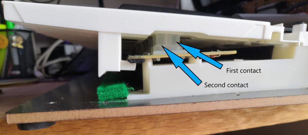
You may remember from part 4 that the circuit board below the keys has two contacts for each key, and the upper contact is closed slightly before the lower contact.

It turns out, this is how some MIDI devices know how hard, or more precisely how fast, we are hitting the keys. This keyboard at least, simply measures the time difference between the first and second contact.

Arduino MIDI velocity in practice

The first thing we should do is get some idea of the range of timings involved.

This is very simple. Arduino provides a function called millis() which tells us the number of milliseconds which have ticked by since power-on.

All we need to do then is store the current value of millis() when the first contact is made, and compare it with the current value on second contact. That will tell us the time difference between the two. This will of course depend on the physical arrangement of the switches relative to the keys.

For my keyboard, no matter how hard (or fast!) I hit the key, I never got a period shorter than 2ms. When trying to press they keys softly, for a normal sort of press, I rarely saw a period longer than 80ms. For now, then, I’m going to assume that I should be loudest with a period of 2ms, and softest with a period of 80ms.

For a simple velocity function, then, we could just calculate a linear relationship between these two. Generally, though, keyboards offer a variety of velocity “curves” which create different effects by having different relationships between key speed and MIDI velocity. The music recording website soundonsound.com has a good explanation of why this is the case.

The generation game

Calculating values along these different curves may be expensive in CPU-cycle terms, and we need to preserve responsiveness to make our keyboard an effective musical instrument. We can’t have calculations slowing down the output of a note when a key is pressed. For this reason, we’re going to precalculate our curves and use look-up tables.

Microsoft Excel is a great tool to use for something like this. We can easily play with different formulae and values, see the curves presented graphically, and then even generate the code we’ll need to include in our program.

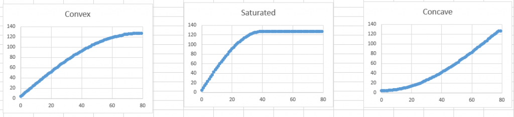
My first attempt at translating the curves from the soundonsound.com article into my own curves was based on “powers” of the speed of the press. This is basically because I thought the Convex graph looked a bit like a graph of the square root of x (x^0.5), and the Concave graph looked a bit like a graph of x squared (x^2). The saturated graph is similar to the convex graph, but saturates at maximum volume beyond a certain threshold. (The actual powers used aren’t 0.5, and 2, I adjusted them to improve the curve shape, but they are similar.)

The graphs looked like this:

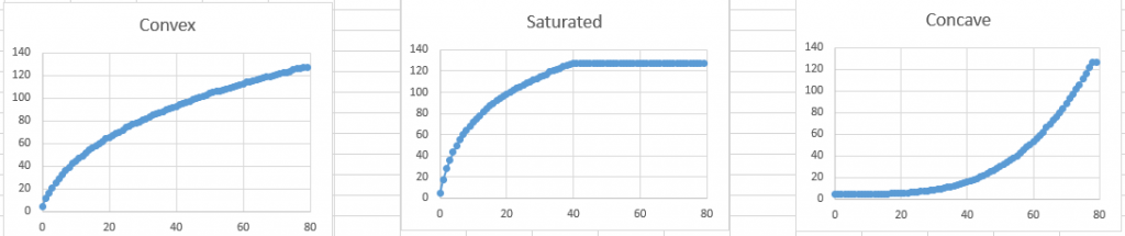
I think the Concave curve looks fine, but for me the Convex curves don’t seem quite right. The saturated curve should have a smoother transition at the threshold. (I’ve omitted the linear curve, surprisingly, it looks like a straight line!)

I then tried curves based on trigonometric functions. Functions based on sin(x) were used for Convex and Saturated, and on 1-cos(x) for Concave. This gave the following graphs:

These Convex curves are much better, but I prefer the original Concave curve, so will stick with that one.

Excel to C

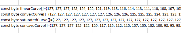
Now I have a spreadsheet containing a list of all the values I want in each array, generating C code to produce them is nice and easy. The latest versions Excel have a new function called TEXTJOIN which allows all of the members of a range of data to be joined together in a string, separated by a given delimiter, a comma in my case.

="const byte " & A103 & "Curve[]={" & TEXTJOIN(", ",TRUE,E$21:E$101) & "};"

So, using a formula like the one above, where “&” just means join together two strings, allows us to generate code which looks this this in Excel, and can be simply copied and pasted into our program:

All we need to do then is to make our program select the correct curve based on a setting, and select the correct element from the array based on the gap between switches.

The Excel sheet in which I did all this is available for download here:

As always, my code is available on github.

Assignable controllers

Fortunately, user settings are something I’ve been working on between blog posts. Without going into too much detail, because it’s out of scope for this post, I have a system in the software which allows any of the 157 different controllable parameters to be easily assigned to the different controls on the control panel. Just like the original keyboard should have done!

The upshot, for now, being that the fourth rotary controller is set up, by default, to select one of our four velocity curves.

So let’s hear that speed!

As you can hear in the video, curve 0, linear, has some volume difference between notes. Curve 1 is the convex curve, which is more compressed. Curve 2 is the saturated convex curve, where we can hear hardly any volume difference at all. The greatest difference, unsurprisingly, is found in the concave curve, number 3, where only very firm pressure generates the loudest notes.

The results above suggest that I might want a little more difference in those other curves – maybe considering gaps up to 80ms is a bit generous – by reducing that I could get more difference in volume with smaller difference in pressure.

Perhaps I’ll try that, which will be easy enough with my Excel method but, for now, this will do.

There is very little left to do now – we have a fully functioning keyboard. I’ve also implemented the settings feature as I mentioned above, so I think we can call this a successful project!